import pandas as pd

url = "https://www.epa.gov/system/files/other-files/2024-06/us-ghg-emissions_fig-1.csv"

from io import StringIO
import pandas as pd
import requests

def url_data_request(url, skiprows):
    headers = {
        "User-Agent": "Mozilla/5.0 (X11; Ubuntu; Linux x86_64; rv:109.0) Gecko/20100101 Firefox/118.0",
    }
    f = StringIO(requests.get(url, headers=headers).text)
    df_url = pd.read_csv(f, skiprows = skiprows)
    return df_url

df = url_data_request(url, 6)14 Greenhouse Gas Emissions
In this section, we will analyze Greenhouse Gas (GHG) emissions.
What are Greenhouse Gases and why do we care about them?
As before, we will rely on EPA or other governmental agencies, multinational agencies or some scientific articles for evidence.
EPA highlights that:
Gases that trap heat in the atmosphere are called greenhouse gases. As greenhouse gas emissions from human activities increase, they build up in the atmosphere and warm the climate, leading to many other changes around the world—in the atmosphere, on land, and in the oceans.
EPA gives detailed information on Greenhouse Gases at https://www.epa.gov/ghgemissions/overview-greenhouse-gases. There main Greenhouse Gases that we will analyze are:
- Carbon dioxide (CO2): Carbon dioxide enters the atmosphere through burning fossil fuels (coal, natural gas, and oil), solid waste, trees and other biological materials, and also as a result of certain chemical reactions (e.g., cement production). Carbon dioxide is removed from the atmosphere (or “sequestered”) when it is absorbed by plants as part of the biological carbon cycle.
- Methane (CH4): Methane is emitted during the production and transport of coal, natural gas, and oil. Methane emissions also result from livestock and other agricultural practices, land use, and by the decay of organic waste in municipal solid waste landfills.
- Nitrous oxide (N2O): Nitrous oxide is emitted during agricultural, land use, and industrial activities; combustion of fossil fuels and solid waste; as well as during treatment of wastewater.
- Fluorinated gases: Hydrofluorocarbons, perfluorocarbons, sulfur hexafluoride, and nitrogen trifluoride are synthetic, powerful greenhouse gases that are emitted from a variety of household, commercial, and industrial applications and processes.
We can see the composition of total GHG emissions as of 2022 for the U.S. from EPA.
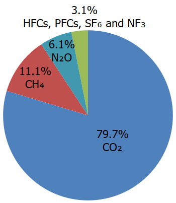
Total U.S. Emissions in 2022 = 6,343 Million Metric Tons of CO₂ equivalent.
14.1 Carbon Dioxide (CO2)
Lets us start with CO2. Why do we care about CO2?
First, CO2 accounts for almost 80% of the Greenhouse Gases.
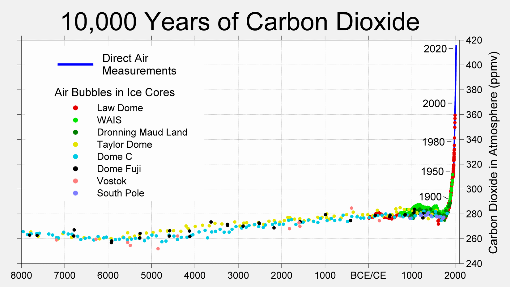
Second, there is a steep increase in the CO2 over the past 10,000 years. The increase over the past 100 years or so is alarming if the trends continue.
Before diving deeper into the sources and causes of CO2 emissions, let us first reproduce the EPA graphs on CO2 emissions.
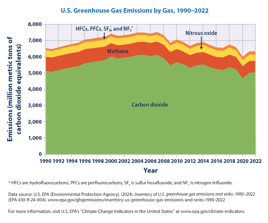
This figure shows emissions of carbon dioxide, methane, nitrous oxide, and several fluorinated gases in the United States from 1990 to 2022. For consistency, emissions are expressed in million metric tons of carbon dioxide equivalents.
We will repeat the steps that we have undertaken in part 1 of the book to reproduce the figure. So, we won’t give detailed explanations as many of these are covered before.
The data for the figure is available at https://www.epa.gov/system/files/other-files/2024-06/us-ghg-emissions_fig-1.csv
What does the code do? As we moved into Part 2 and AI agents have become much better, we can ask Copilot to explain the code. We edited the explanation to make it shorter.
The provided code snippet is written in Python and is used to fetch and process a CSV file from a given URL.
The code begins by importing the necessary libraries. The pandas library is imported twice, which is redundant, but it is a powerful data manipulation library used to handle the CSV data.
- Our mistake! We missed it, but Copilot doesn’t! There is no harm in importing twice but it is redundant.
The StringIO class from the io module is imported to handle string data as file-like objects, and the requests library is imported to make HTTP requests.
The URL of the CSV file is stored in the variable url. This URL points to a CSV file hosted on the EPA’s website, which contains data on U.S. greenhouse gas emissions.
A function named url_data_request is defined to fetch and process the CSV data from the URL. This function takes two parameters: url and skiprows.
- The url parameter is the URL of the CSV file, and skiprows specifies the number of rows to skip at the beginning of the file.
- This is useful for skipping metadata or header information that is not part of the actual data.
Inside the function, a dictionary named headers is defined to mimic a web browser’s request. This is done to avoid potential issues with web servers that block requests from non-browser clients.
The requests.get function is used to fetch the content of the URL, and the response text is passed to StringIO to create a file-like object. This object is then read into a Pandas DataFrame using the pd.read_csv function, with the skiprows parameter to skip the specified number of rows.
Finally, the function returns the DataFrame containing the CSV data.
The url_data_request function is called with the URL and skiprows set to 6, and the resulting DataFrame is stored in the variable df.
This DataFrame now contains the processed data from the CSV file, ready for further analysis or visualization.
As you can see, the explanation is more detailed and useful than what we would have written. So we decided to use it, with some minor edits.
As before, the first step with any dataset is always to get some basic info.
We can see from df.shape that there are 33 rows and 5 variables.
We can do descriptive stats on the numerical variables.
| Year | Methane | Nitrous oxide | HFCs, PFCs, SF6, and NF3 | |
|---|---|---|---|---|
| count | 33.00000 | 33.000000 | 33.000000 | 33.000000 |
| mean | 2006.00000 | 802.654633 | 417.133412 | 163.509376 |
| std | 9.66954 | 47.816996 | 13.205529 | 20.770491 |
| min | 1990.00000 | 702.354745 | 389.707858 | 118.265427 |
| 25% | 1998.00000 | 764.386625 | 410.943810 | 155.868137 |
| 50% | 2006.00000 | 806.645870 | 419.175093 | 169.045426 |
| 75% | 2014.00000 | 835.477487 | 423.413845 | 176.571344 |
| max | 2022.00000 | 879.645413 | 439.607792 | 198.128038 |
As we can see, the data is from 1990-2022 and includes emissions data on methane, nitrous oxide, and several fluorinated gases in the United States (re expressed in million metric tons of carbon dioxide equivalents).
That’s only 4 variables or columns, including year. Where did the fifth column go?
We should have first checked the data types in the dataset.
Year                          int64
Carbon dioxide               object
Methane                     float64
Nitrous oxide               float64
HFCs, PFCs, SF6, and NF3    float64
dtype: object
We can see that Carbon dioxide (CO2) is an object and that’s why the df.describe() didn’t give descriptive statistics on it.
Why is it an object type? We have no idea!
Looking at the data, all the values look numerical.
| Year | Carbon dioxide | Methane | Nitrous oxide | HFCs, PFCs, SF6, and NF3 | |
|---|---|---|---|---|---|
| 0 | 1990 | 5,131.65 | 871.658825 | 408.151400 | 125.454537 |
| 1 | 1991 | 5,076.30 | 879.645413 | 398.477140 | 118.265427 |
| 2 | 1992 | 5,178.73 | 877.381636 | 397.294008 | 122.945240 |
| 3 | 1993 | 5,279.48 | 864.852491 | 418.461318 | 123.662121 |
| 4 | 1994 | 5,361.82 | 873.401867 | 419.175093 | 128.238674 |
| 5 | 1995 | 5,425.80 | 866.586056 | 423.495394 | 146.256594 |
| 6 | 1996 | 5,601.06 | 861.737879 | 435.519013 | 157.943424 |
| 7 | 1997 | 5,673.11 | 847.921716 | 419.608268 | 168.341026 |
| 8 | 1998 | 5,736.33 | 835.477487 | 423.373150 | 183.810398 |
| 9 | 1999 | 5,800.25 | 815.812634 | 418.744132 | 183.826627 |
| 10 | 2000 | 6,023.13 | 815.701845 | 410.943810 | 170.107309 |
| 11 | 2001 | 5,903.53 | 807.084109 | 421.725702 | 154.972910 |
| 12 | 2002 | 5,947.79 | 801.091353 | 422.934556 | 158.077394 |
| 13 | 2003 | 6,006.42 | 801.128955 | 423.413845 | 155.928303 |
| 14 | 2004 | 6,111.52 | 796.433638 | 428.505590 | 155.868137 |
| 15 | 2005 | 6,126.86 | 795.429181 | 419.189952 | 153.153855 |
| 16 | 2006 | 6,045.30 | 806.645870 | 420.562160 | 156.667115 |
| 17 | 2007 | 6,121.52 | 810.254941 | 431.642027 | 166.486877 |
| 18 | 2008 | 5,919.21 | 821.582197 | 416.514826 | 169.045426 |
| 19 | 2009 | 5,486.09 | 806.775967 | 410.066543 | 163.987454 |
| 20 | 2010 | 5,668.74 | 807.598702 | 418.263291 | 171.403236 |
| 21 | 2011 | 5,540.33 | 778.288480 | 419.850882 | 173.296084 |
| 22 | 2012 | 5,332.81 | 764.063618 | 392.793611 | 171.237077 |
| 23 | 2013 | 5,473.66 | 766.205413 | 434.022492 | 171.519475 |
| 24 | 2014 | 5,529.88 | 762.391457 | 439.607792 | 173.968019 |
| 25 | 2015 | 5,368.29 | 764.386625 | 426.965957 | 176.571344 |
| 26 | 2016 | 5,246.40 | 744.590524 | 413.408295 | 175.634227 |
| 27 | 2017 | 5,196.54 | 759.480075 | 417.818944 | 177.188295 |
| 28 | 2018 | 5,362.19 | 771.481067 | 439.453215 | 179.624212 |
| 29 | 2019 | 5,234.49 | 754.341139 | 416.377483 | 184.922055 |
| 30 | 2020 | 4,688.97 | 735.348832 | 391.167731 | 186.321505 |
| 31 | 2021 | 5,017.20 | 720.468152 | 398.167133 | 192.956988 |
| 32 | 2022 | 5053.018689 | 702.354745 | 389.707858 | 198.128038 |
All the values are included with two decimals whereas the value for 2022 has 6 decimals. We suspect this may be an issue. But we don’t know.
AI is smart but real world is messy! There are always some cases where the data is slightly different or there is some nuance that makes the AI generated code not work. So, it is still useful to learn and understand coding!
Let us read object type as a float type variable.
Unfortunately, it doesn’t work :(
We get an error.
 ---------------------------------------------------------------------------
ValueError                                Traceback (most recent call last)
Cell In[19], line 1
----> 1 df['Carbon dioxide'] = df['Carbon dioxide'].astype(float)

File /usr/local/lib/python3.11/site-packages/pandas/core/generic.py:6324, in NDFrame.astype(self, dtype, copy, errors)
   6317     results = [
   6318         self.iloc[:, i].astype(dtype, copy=copy)
   6319         for i in range(len(self.columns))
   6320     ]
   6322 else:
   6323     # else, only a single dtype is given
-> 6324     new_data = self._mgr.astype(dtype=dtype, copy=copy, errors=errors)
   6325     return self._constructor(new_data).__finalize__(self, method="astype")
   6327 # GH 33113: handle empty frame or series

File /usr/local/lib/python3.11/site-packages/pandas/core/internals/managers.py:451, in BaseBlockManager.astype(self, dtype, copy, errors)
    448 elif using_copy_on_write():
    449     copy = False
--> 451 return self.apply(
    452     "astype",
    453     dtype=dtype,
    454     copy=copy,
    455     errors=errors,
    456     using_cow=using_copy_on_write(),
    457 )

File /usr/local/lib/python3.11/site-packages/pandas/core/internals/managers.py:352, in BaseBlockManager.apply(self, f, align_keys, **kwargs)
    350         applied = b.apply(f, **kwargs)
    351     else:
--> 352         applied = getattr(b, f)(**kwargs)
    353     result_blocks = extend_blocks(applied, result_blocks)
    355 out = type(self).from_blocks(result_blocks, self.axes)

File /usr/local/lib/python3.11/site-packages/pandas/core/internals/blocks.py:511, in Block.astype(self, dtype, copy, errors, using_cow)
    491 """
    492 Coerce to the new dtype.
    493
   (...)
    507 Block
    508 """
    509 values = self.values
--> 511 new_values = astype_array_safe(values, dtype, copy=copy, errors=errors)
    513 new_values = maybe_coerce_values(new_values)
    515 refs = None

File /usr/local/lib/python3.11/site-packages/pandas/core/dtypes/astype.py:242, in astype_array_safe(values, dtype, copy, errors)
    239     dtype = dtype.numpy_dtype
    241 try:
--> 242     new_values = astype_array(values, dtype, copy=copy)
    243 except (ValueError, TypeError):
    244     # e.g. _astype_nansafe can fail on object-dtype of strings
    245     #  trying to convert to float
    246     if errors == "ignore":

File /usr/local/lib/python3.11/site-packages/pandas/core/dtypes/astype.py:187, in astype_array(values, dtype, copy)
    184     values = values.astype(dtype, copy=copy)
    186 else:
--> 187     values = _astype_nansafe(values, dtype, copy=copy)
    189 # in pandas we don't store numpy str dtypes, so convert to object
    190 if isinstance(dtype, np.dtype) and issubclass(values.dtype.type, str):

File /usr/local/lib/python3.11/site-packages/pandas/core/dtypes/astype.py:138, in _astype_nansafe(arr, dtype, copy, skipna)
    134     raise ValueError(msg)
    136 if copy or is_object_dtype(arr.dtype) or is_object_dtype(dtype):
    137     # Explicit copy, or required since NumPy can't view from / to object.
--> 138     return arr.astype(dtype, copy=True)
    140 return arr.astype(dtype, copy=copy)

ValueError: could not convert string to float: '5,131.65'
Didn’t we say real world data is messy!!!
We have to do some snooping but it appears that 5,131.65 is a read as a string, for whatever reason.
Now that we know there are some values of ‘Carbon dioxide’ column / variable stored as ‘string’, we can do some data cleaning.
Basically, we removed commas and leading and trailing empty spaced and then read the string as a float.
Did it work? Let us check!
| Year | Carbon dioxide | Methane | Nitrous oxide | HFCs, PFCs, SF6, and NF3 | |
|---|---|---|---|---|---|
| count | 33.00000 | 33.000000 | 33.000000 | 33.000000 | 33.000000 |
| mean | 2006.00000 | 5535.406627 | 802.654633 | 417.133412 | 163.509376 |
| std | 9.66954 | 377.903314 | 47.816996 | 13.205529 | 20.770491 |
| min | 1990.00000 | 4688.970000 | 702.354745 | 389.707858 | 118.265427 |
| 25% | 1998.00000 | 5246.400000 | 764.386625 | 410.943810 | 155.868137 |
| 50% | 2006.00000 | 5486.090000 | 806.645870 | 419.175093 | 169.045426 |
| 75% | 2014.00000 | 5903.530000 | 835.477487 | 423.413845 | 176.571344 |
| max | 2022.00000 | 6126.860000 | 879.645413 | 439.607792 | 198.128038 |
Now, we see descriptive statistics for ‘Carbon dioxide’ also! The code worked!!
It is easy to plot these using Plotly.
Let us focus on ‘Carbon dioxide’ so that we can see if there are significant increases over time.
import plotly.express as px

fig = px.line(df, x='Year', y=['Carbon dioxide'],
              labels={'value': 'Emissions (million metric tons of CO2 equivalents)', 'variable': 'Gas'},
              title='CO2 Emissions Over Time')

fig.update_layout(
    yaxis_title="Emissions (million metric tons of CO2 equivalents)",
    xaxis_title="Year",
    title_x=0.5,
    hovermode="x",
    legend=dict(title="CO2 Emissions", x=0.2, y=0.3)
)
fig.show()
Now, we can see that the CO2 emissions steadily increased from 1990 to 2007 or so but decreased later and now at around the 1990 levels. Scale matters for graphing!
14.2 Other GHG Emissions
Let us see the other GHG that are at a different scale than CO2 (that accounts for approximately 80% of the GHG emissions)
import plotly.express as px

fig = px.line(df, x='Year', y=['Carbon dioxide', 'Methane', 'Nitrous oxide', 'HFCs, PFCs, SF6, and NF3'],
              labels={'value': 'Emissions (million metric tons of CO2 equivalents)', 'variable': 'Gas'},
              title='Greenhouse Gas Emissions Over Time')

fig.update_layout(
    yaxis_title="Emissions (million metric tons of CO2 equivalents)",
    xaxis_title="Year",
    title_x=0.5,
    hovermode="x",
    legend=dict(title="GhG Emissions", x=0.2, y=0.3)
)

fig.show()
This graph is not as useful as ‘Carbon dioxide’ emissions dominate and relative to that, every other gas emission seems smaller.
We can just focus on other GHG gases in the figure to see the trends clearly.
import plotly.express as px

fig = px.line(df, x='Year', y=['Methane', 'Nitrous oxide', 'HFCs, PFCs, SF6, and NF3'],
              labels={'value': 'Emissions (million metric tons of CO2 equivalents)', 'variable': 'Gas'},
              title='Greenhouse Gas Emissions Over Time')

fig.update_layout(
    yaxis_title="Emissions (million metric tons of CO2 equivalents)",
    xaxis_title="Year",
    title_x=0.5,
    hovermode="x",
    legend=dict(title="GhG Emissions", x=0.1, y=0.8)
)
fig.show()
We see that ‘Nitrous Oxide’ is more or less stable over the period 1990-2022.
‘HFCs’ seem to have increased over the 1990-2022 time period.
Now that we see the different GhG emissions on different scales, let us combine them.
import plotly.express as px

fig = px.area(df, x='Year', y=['Carbon dioxide', 'Methane', 'Nitrous oxide', 'HFCs, PFCs, SF6, and NF3'],
              labels={'value': 'Emissions (million metric tons of CO2 equivalents)', 'variable': 'Gas'},
              title='Greenhouse Gas Emissions Over Time')

fig.update_layout(
    yaxis_title="Emissions (million metric tons of CO2 equivalents)",
    xaxis_title="Year",
    title_x=0.5,
    hovermode="x",
    legend=dict(title="GhG Emissions", x=0.3, y=0.3)
)
fig.show()
Now we see a graph that looks more like the Figure 1 from EPA for GHG emissions.
What are the key insights from this figure? EPA states:
In 2022, U.S. greenhouse gas emissions totaled 6,343 million metric tons (14.0 trillion pounds) of carbon dioxide equivalents. This total represents a 3.0 percent decrease since 1990, down from a high of 15.2 percent above 1990 levels in 2007. The sharp decline in emissions from 2019 to 2020 was largely due to the impacts of the coronavirus (COVID-19) pandemic on travel and economic activity. Emissions increased from 2020 to 2022 by 5.7 percent, driven largely by an increase in carbon dioxide emissions from fossil fuel combustion due to economic activity rebounding after the height of the pandemic (Figure 1).
For the United States, during the period from 1990 to 2022 (Figure 1): - Emissions of carbon dioxide, the primary greenhouse gas emitted by human activities, decreased by 2 percent. - Methane emissions decreased by 19 percent, as reduced emissions from landfills, coal mines, and natural gas systems more than offset increases in emissions from activities such as livestock production. - Nitrous oxide emissions, predominantly from agricultural soil management practices such as the use of nitrogen as a fertilizer, decreased by 5 percent. - Emissions of fluorinated gases (hydrofluorocarbons, perfluorocarbons, sulfur hexafluoride, and nitrogen trifluoride), released as a result of commercial, industrial, and household uses, increased by 58 percent.
14.3 U.S. Greenhouse Gas Emissions and Sinks by Economic Sector, 1990–2022
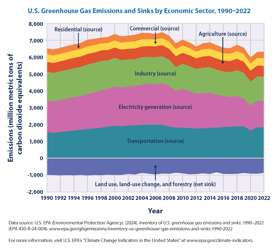
EPA also plots the sourcs of U.S. Greenhouse Gas Emissions and Sinks by Economic Sector, 1990–2022.
Per the EPA,
This figure shows greenhouse gas emissions and sinks (negative values) by source in the United States from 1990 to 2022. For consistency, emissions are expressed in million metric tons of carbon dioxide equivalents. All electric power emissions are grouped together in the “Electric power” sector, so other sectors such as “Residential” and “Commercial” are only showing non-electric sources, such as burning oil or gas for heating. Totals do not match Figure 1 exactly because the economic sectors shown here do not include emissions from U.S. territories outside the 50 states.
Let us look at the sector wise contribution. Note the units are million metric tons of CO2 equivalents.
Before going into generating figures, we want to highlight how messy the real world data can be and how it can change from year to year, even it is from the exact same source.
While revising this version of the book, we have realized that the data has been updated from the 2022-07 version to 2024-06.
The nice thing with coding is that we just need to change the link. But we will first use the old link to highlight the importance of data cleaning issues.
Note, this is not the latest data but the July 2022 version of the data for Figure 2 in EPA U.S. GHG emissions.
Let us read the data as usual
As before, the first step with any dataset is always to get some basic info.
We can see from df.shape that there are 31 rows and 8 variables.
Index(['Unnamed: 0', 'Transportation', 'Electricity generation', 'Industry',
       'Agriculture', 'Commercial', 'Residential',
       'Land use, land-use change, and forestry (net sink)'],
      dtype='object')
We notice that the first column, Year is read as ‘Unnamed: 0’. Let us see if we notice anything else that is not what we expect
<class 'pandas.core.frame.DataFrame'>
RangeIndex: 31 entries, 0 to 30
Data columns (total 8 columns):
 #   Column                                              Non-Null Count  Dtype
---  ------                                              --------------  -----
 0   Unnamed: 0                                          31 non-null     int64
 1   Transportation                                      31 non-null     float64
 2   Electricity generation                              31 non-null     float64
 3   Industry                                            31 non-null     float64
 4   Agriculture                                         31 non-null     float64
 5   Commercial                                          31 non-null     float64
 6   Residential                                         31 non-null     float64
 7   Land use, land-use change, and forestry (net sink)  31 non-null     object
dtypes: float64(6), int64(1), object(1)
memory usage: 2.1+ KB
Land use, land-use change, and forestry (net sink) is read as an object. It suggests that the column may be read with different data types. So let us look at the data quickly to see what is happening.
| Unnamed: 0 | Transportation | Electricity generation | Industry | Agriculture | Commercial | Residential | Land use, land-use change, and forestry (net sink) | |
|---|---|---|---|---|---|---|---|---|
| 0 | 1990 | 1526.434289 | 1880.548218 | 1652.361348 | 596.778204 | 427.109795 | 345.070789 | -860.6250574 |
| 1 | 1991 | 1480.303906 | 1874.832994 | 1625.461259 | 587.493379 | 434.321072 | 354.689750 | -869.9082889 |
| 2 | 1992 | 1539.881716 | 1890.103637 | 1662.343992 | 588.301071 | 429.939070 | 361.222025 | -862.4402032 |
| 3 | 1993 | 1576.887693 | 1965.574487 | 1631.906633 | 616.367720 | 423.366758 | 372.612499 | -844.206428 |
| 4 | 1994 | 1631.842860 | 1990.300202 | 1657.477536 | 603.473044 | 426.583160 | 363.260147 | -857.5259735 |
| 5 | 1995 | 1667.019780 | 2006.877479 | 1675.133984 | 615.669467 | 425.696364 | 367.523521 | -831.7775006 |
| 6 | 1996 | 1723.249166 | 2079.434226 | 1705.045256 | 622.907953 | 433.307228 | 399.454803 | -852.1428676 |
| 7 | 1997 | 1749.849330 | 2144.903577 | 1705.172770 | 611.328521 | 425.795877 | 380.828659 | -833.4407232 |
| 8 | 1998 | 1792.295978 | 2231.446285 | 1677.755098 | 618.246994 | 400.541006 | 346.873254 | -835.2578601 |
| 9 | 1999 | 1863.292087 | 2244.837093 | 1627.052157 | 609.289744 | 396.926502 | 366.684458 | -828.0496898 |
| 10 | 2000 | 1913.550780 | 2351.125685 | 1616.991263 | 594.854300 | 411.195289 | 387.992539 | -825.2288316 |
| 11 | 2001 | 1885.434887 | 2311.387024 | 1569.909847 | 615.526557 | 400.209078 | 378.076884 | -828.8079892 |
| 12 | 2002 | 1925.980857 | 2326.759449 | 1550.961500 | 618.674248 | 401.730691 | 375.286669 | -790.5485356 |
| 13 | 2003 | 1933.326749 | 2357.952283 | 1529.061153 | 618.962290 | 417.965117 | 393.728943 | -820.7858422 |
| 14 | 2004 | 1965.852074 | 2390.768614 | 1577.981113 | 631.722629 | 415.777828 | 381.852435 | -729.4523162 |
| 15 | 2005 | 1975.495129 | 2456.737090 | 1536.176420 | 626.253214 | 405.442432 | 371.015529 | -789.7931676 |
| 16 | 2006 | 1975.865366 | 2401.231383 | 1570.640402 | 625.786501 | 391.901762 | 334.309400 | -817.1760559 |
| 17 | 2007 | 1974.426677 | 2467.226239 | 1560.386569 | 642.720748 | 405.856004 | 355.254855 | -776.3550104 |
| 18 | 2008 | 1870.906050 | 2414.114945 | 1501.553646 | 631.031054 | 413.166512 | 363.906982 | -766.4712252 |
| 19 | 2009 | 1796.295049 | 2198.273322 | 1345.926535 | 632.860470 | 416.903785 | 354.545147 | -73448.90% |
| 20 | 2010 | 1802.276352 | 2313.956993 | 1438.778760 | 641.029259 | 419.290316 | 355.539184 | -761.0363768 |
| 21 | 2011 | 1768.595360 | 2211.767283 | 1443.335476 | 622.717221 | 415.067661 | 349.093809 | -800.7290152 |
| 22 | 2012 | 1748.912232 | 2073.785620 | 1440.040968 | 606.452578 | 396.025010 | 306.943124 | -799.9251081 |
| 23 | 2013 | 1751.515531 | 2092.343183 | 1489.536433 | 645.157276 | 419.341960 | 357.731086 | -767.4142623 |
| 24 | 2014 | 1785.407074 | 2092.532800 | 1474.546661 | 654.114340 | 429.600526 | 378.276992 | -781.3816316 |
| 25 | 2015 | 1793.399368 | 1952.725752 | 1464.017871 | 656.101038 | 442.084720 | 351.469522 | -700.0664105 |
| 26 | 2016 | 1828.045564 | 1860.497992 | 1424.355203 | 643.420271 | 426.906642 | 327.812635 | -826.6421699 |
| 27 | 2017 | 1845.162609 | 1780.552030 | 1446.687191 | 644.395728 | 428.486050 | 329.880970 | -781.2093236 |
| 28 | 2018 | 1874.726295 | 1799.826648 | 1507.647460 | 657.914982 | 444.233499 | 377.368858 | -769.266566 |
| 29 | 2019 | 1874.291137 | 1650.961498 | 1521.665941 | 663.895669 | 452.139788 | 384.178158 | -730.4876898 |
| 30 | 2020 | 1627.618555 | 1482.182865 | 1426.194536 | 635.105961 | 425.312514 | 361.952257 | -758.9433076 |
We can immediately see that 2009 for Land use, land-use change, and forestry (net sink) is -73448.90%. For some reason, it is read as a ‘%’ and the value needs to be adjusted by a factor of 100.
There are never any clean data sets! We need to clean the data ourselves many a time. Let us get to it.
| Unnamed: 0 | Transportation | Electricity generation | Industry | Agriculture | Commercial | Residential | |
|---|---|---|---|---|---|---|---|
| count | 31.000000 | 31.000000 | 31.000000 | 31.000000 | 31.000000 | 31.000000 | 31.000000 |
| mean | 2005.000000 | 1789.294855 | 2106.308610 | 1550.196935 | 625.114595 | 419.426581 | 362.401157 |
| std | 9.092121 | 138.775245 | 252.071204 | 96.760250 | 20.358572 | 14.814310 | 20.424532 |
| min | 1990.000000 | 1480.303906 | 1482.182865 | 1345.926535 | 587.493379 | 391.901762 | 306.943124 |
| 25% | 1997.500000 | 1736.080699 | 1921.414694 | 1469.282266 | 613.427539 | 408.525647 | 353.007335 |
| 50% | 2005.000000 | 1796.295049 | 2092.532800 | 1550.961500 | 622.907953 | 419.341960 | 363.260147 |
| 75% | 2012.500000 | 1880.080591 | 2320.358221 | 1629.479395 | 641.875004 | 427.797922 | 377.722871 |
| max | 2020.000000 | 1975.865366 | 2467.226239 | 1705.172770 | 663.895669 | 452.139788 | 399.454803 |
df.rename(columns={'Unnamed: 0': "Year"}, inplace = True)

#for some reason, 2009 data for "Land use, .." has an extra % that is creating issues;
df['Land use, land-use change, and forestry (net sink)'] = df['Land use, land-use change, and forestry (net sink)'].astype("str")

# # need to remove % manually or through regex for 2009
df['Land use, land-use change, and forestry (net sink)'] = df['Land use, land-use change, and forestry (net sink)'].str.replace('%','')

df['Land use, land-use change, and forestry (net sink)'] = df['Land use, land-use change, and forestry (net sink)'].astype("float")

# divide the specific value by 100 as it was in % before
df.loc[(df['Year'] == 2009), 'Land use, land-use change, and forestry (net sink)'] = df.loc[(df['Year'] == 2009), 'Land use, land-use change, and forestry (net sink)']*0.01
Let us unpack the code step-by-step:
- We renamed the column ‘Unnamed: 0’ to ‘Year’. The inplace=True parameter ensures that the change is made directly to the DataFrame df without needing to reassign it.
- We converted the ‘Land use, land-use change, and forestry (net sink)’ column to a string type. This is necessary because the next operation involves string manipulation.
- We removed any ‘%’ characters from the ‘Land use, land-use change, and forestry (net sink)’ column. The str.replace(‘%’, ’‘) method is used to replace’%’ with an empty string.
- We converted the ‘Land use, land-use change, and forestry (net sink)’ column back to a float type. This is necessary for numerical operations.
- We select the rows where the ‘Year’ is 2009 df.loc[(df[‘Year’] == 2009)]) and adjust the ‘Land use, land-use change, and forestry (net sink)’ values by dividing them by 100. This is because the original value was in percentage form.
We can do descriptive stats on the numerical variables.
| Year | Transportation | Electricity generation | Industry | Agriculture | Commercial | Residential | Land use, land-use change, and forestry (net sink) | |
|---|---|---|---|---|---|---|---|---|
| count | 31.000000 | 31.000000 | 31.000000 | 31.000000 | 31.000000 | 31.000000 | 31.000000 | 31.000000 |
| mean | 2005.000000 | 1789.294855 | 2106.308610 | 1550.196935 | 625.114595 | 419.426581 | 362.401157 | -801.018853 |
| std | 9.092121 | 138.775245 | 252.071204 | 96.760250 | 20.358572 | 14.814310 | 20.424532 | 44.477461 |
| min | 1990.000000 | 1480.303906 | 1482.182865 | 1345.926535 | 587.493379 | 391.901762 | 306.943124 | -869.908289 |
| 25% | 1997.500000 | 1736.080699 | 1921.414694 | 1469.282266 | 613.427539 | 408.525647 | 353.007335 | -832.609112 |
| 50% | 2005.000000 | 1796.295049 | 2092.532800 | 1550.961500 | 622.907953 | 419.341960 | 363.260147 | -800.729015 |
| 75% | 2012.500000 | 1880.080591 | 2320.358221 | 1629.479395 | 641.875004 | 427.797922 | 377.722871 | -768.340414 |
| max | 2020.000000 | 1975.865366 | 2467.226239 | 1705.172770 | 663.895669 | 452.139788 | 399.454803 | -700.066410 |
Now, we have all the variables in numerical format, we can use plotly to plot the figures.
However, things are never this simple. We reran the code and updated the dataset in the latest revision (August 2024).
It appeared that all we had to do was change the URL to reflect the updated data.
Let us look at this updated data.
<class 'pandas.core.frame.DataFrame'>
RangeIndex: 33 entries, 0 to 32
Data columns (total 8 columns):
 #   Column                                              Non-Null Count  Dtype
---  ------                                              --------------  -----
 0   Unnamed: 0                                          33 non-null     int64
 1   Transportation                                      33 non-null     object
 2   Electric power industry                             33 non-null     object
 3   Industry                                            33 non-null     object
 4   Agriculture                                         33 non-null     float64
 5   Commercial                                          33 non-null     float64
 6   Residential                                         33 non-null     float64
 7   Land use, land-use change, and forestry (net sink)  33 non-null     float64
dtypes: float64(4), int64(1), object(3)
memory usage: 2.2+ KB
Now, we notice that ‘Land use, land-use change, and forestry (net sink)’ are in float64 numerical format but some other variables like ‘Transportation’, ‘Electric power industry’ and ‘Industry’ are in object data type. These were all float64 data type in the 2022 version of the data.
Our code would have given errors because we wouldn’t have been able to plot these variables.
There is always some changes to the data or data structure and it is always useful to check the data before running visualization or analysis code.
What seems to be the issue?
| Unnamed: 0 | Transportation | Electric power industry | Industry | Agriculture | Commercial | Residential | Land use, land-use change, and forestry (net sink) | |
|---|---|---|---|---|---|---|---|---|
| 0 | 1990 | 1,521.42 | 1,880.18 | 1,723.32 | 595.946054 | 447.006292 | 345.597115 | -976.694756 |
| 1 | 1991 | 1,474.77 | 1,874.41 | 1,702.87 | 587.411997 | 454.452721 | 355.264350 | -988.981068 |
| 2 | 1992 | 1,533.76 | 1,889.64 | 1,729.28 | 587.511141 | 449.970155 | 361.808133 | -1007.385245 |
| 3 | 1993 | 1,570.22 | 1,964.99 | 1,701.00 | 608.733193 | 443.082240 | 373.147538 | -991.346525 |
| 4 | 1994 | 1,624.55 | 1,989.60 | 1,719.67 | 612.158538 | 446.051460 | 363.773428 | -1005.221528 |
| 5 | 1995 | 1,659.12 | 2,006.05 | 1,741.77 | 618.123912 | 444.491719 | 367.292045 | -980.231228 |
| 6 | 1996 | 1,714.59 | 2,078.44 | 1,762.11 | 625.693883 | 451.625773 | 399.137915 | -1011.174579 |
| 7 | 1997 | 1,740.50 | 2,143.76 | 1,765.41 | 610.728830 | 442.880099 | 380.425938 | -985.194814 |
| 8 | 1998 | 1,782.67 | 2,230.09 | 1,757.76 | 621.023100 | 416.338725 | 346.522958 | -996.334680 |
| 9 | 1999 | 1,853.62 | 2,243.49 | 1,703.94 | 614.986761 | 411.817874 | 366.325388 | -968.475616 |
| 10 | 2000 | 1,903.74 | 2,350.06 | 1,699.09 | 607.226572 | 425.633761 | 387.642129 | -983.687718 |
| 11 | 2001 | 1,875.44 | 2,310.78 | 1,631.35 | 622.405680 | 414.052081 | 377.790426 | -979.752372 |
| 12 | 2002 | 1,916.20 | 2,326.47 | 1,613.80 | 628.402932 | 415.310841 | 375.113216 | -924.826536 |
| 13 | 2003 | 1,923.66 | 2,357.97 | 1,593.64 | 627.684215 | 431.720081 | 393.678826 | -957.908300 |
| 14 | 2004 | 1,956.16 | 2,391.13 | 1,639.83 | 633.535447 | 429.132623 | 381.913394 | -860.183752 |
| 15 | 2005 | 1,965.92 | 2,457.45 | 1,587.26 | 634.303237 | 418.863933 | 371.189484 | -907.696609 |
| 16 | 2006 | 1,966.34 | 2,402.37 | 1,624.49 | 638.728891 | 404.901417 | 334.363826 | -951.935738 |
| 17 | 2007 | 1,967.19 | 2,468.32 | 1,611.63 | 654.903372 | 418.425064 | 355.266743 | -900.321359 |
| 18 | 2008 | 1,863.44 | 2,415.24 | 1,571.71 | 643.038956 | 425.324512 | 363.827773 | -912.806240 |
| 19 | 2009 | 1,789.02 | 2,198.66 | 1,415.50 | 639.829854 | 428.256574 | 353.866061 | -850.877697 |
| 20 | 2010 | 1,795.15 | 2,313.10 | 1,488.57 | 647.142320 | 430.587609 | 355.005227 | -886.324754 |
| 21 | 2011 | 1,762.38 | 2,210.22 | 1,488.39 | 641.226366 | 425.528968 | 348.859719 | -941.730797 |
| 22 | 2012 | 1,743.52 | 2,072.66 | 1,473.16 | 624.385259 | 406.456125 | 306.480072 | -929.233916 |
| 23 | 2013 | 1,746.77 | 2,090.99 | 1,533.83 | 658.485864 | 429.200747 | 357.202066 | -886.612352 |
| 24 | 2014 | 1,780.99 | 2,091.04 | 1,526.88 | 660.868014 | 439.358052 | 377.618245 | -923.660383 |
| 25 | 2015 | 1,789.41 | 1,951.70 | 1,506.06 | 657.352663 | 451.674786 | 350.689960 | -820.192444 |
| 26 | 2016 | 1,824.49 | 1,859.33 | 1,456.23 | 650.363698 | 435.630707 | 327.026529 | -916.798491 |
| 27 | 2017 | 1,841.92 | 1,779.36 | 1,478.41 | 658.503899 | 437.389191 | 329.161536 | -926.002254 |
| 28 | 2018 | 1,871.61 | 1,799.18 | 1,541.87 | 683.533939 | 453.481029 | 376.819523 | -915.499704 |
| 29 | 2019 | 1,874.55 | 1,650.75 | 1,531.80 | 661.035227 | 462.630952 | 384.210676 | -863.576006 |
| 30 | 2020 | 1,625.28 | 1,482.17 | 1,435.91 | 640.048676 | 436.915126 | 358.042212 | -904.394729 |
| 31 | 2021 | 1,805.47 | 1,584.45 | 1,455.80 | 645.876462 | 443.663063 | 369.609906 | -910.553723 |
| 32 | 2022 | 1801.520909 | 1577.493448 | 1452.536166 | 633.964509 | 463.661569 | 391.301657 | -854.238577 |
A quick look at the data shows that these variables have two decimals for every year except for 2022. Can this probably be the issue? In 2020, we see that these same variables always have a precision of 4 decimals. Can this be causing the variables to be read as an object now?
| Unnamed: 0 | Agriculture | Commercial | Residential | Land use, land-use change, and forestry (net sink) | |
|---|---|---|---|---|---|
| count | 33.00000 | 33.000000 | 33.000000 | 33.000000 | 33.000000 |
| mean | 2006.00000 | 632.580711 | 434.409572 | 363.211334 | -933.934985 |
| std | 9.66954 | 22.453809 | 15.853136 | 20.528880 | 51.739532 |
| min | 1990.00000 | 587.411997 | 404.901417 | 306.480072 | -1011.174579 |
| 25% | 1998.00000 | 618.123912 | 425.324512 | 353.866061 | -980.231228 |
| 50% | 2006.00000 | 633.964509 | 435.630707 | 363.827773 | -926.002254 |
| 75% | 2014.00000 | 647.142320 | 446.051460 | 377.618245 | -904.394729 |
| max | 2022.00000 | 683.533939 | 463.661569 | 399.137915 | -820.192444 |
We can’t use these variables in plotly until we make them numeric variables.
Thankfully, we just need to modify our old code slightly to adjust for these changes in data.
It looks like this is not the issue! We get an error!
    1,584.45    1,455.80    645.876462  443.663063  369.609906  -910.553723
32  2022    1801.520909 1577.493448 1452.536166 633.964509  463.661569  391.301657  -854.238577
---------------------------------------------------------------------------
ValueError                                Traceback (most recent call last)
File /Users/sc/Library/CloudStorage/GoogleDrive-nextgen360ga@gmail.com/My Drive/NextGen_Web/Climate_P1/Chapters/Part2/GHG.qmd:2
----> 1 df['Transportation'] = df['Transportation'].astype("float")

File /usr/local/lib/python3.11/site-packages/pandas/core/generic.py:6324, in NDFrame.astype(self, dtype, copy, errors)
   6317     results = [
   6318         self.iloc[:, i].astype(dtype, copy=copy)
   6319         for i in range(len(self.columns))
   6320     ]
   6322 else:
   6323     # else, only a single dtype is given
-> 6324     new_data = self._mgr.astype(dtype=dtype, copy=copy, errors=errors)
   6325     return self._constructor(new_data).__finalize__(self, method="astype")
   6327 # GH 33113: handle empty frame or series

File /usr/local/lib/python3.11/site-packages/pandas/core/internals/managers.py:451, in BaseBlockManager.astype(self, dtype, copy, errors)
    448 elif using_copy_on_write():
    449     copy = False
--> 451 return self.apply(
    452     "astype",
    453     dtype=dtype,
    454     copy=copy,
    455     errors=errors,
    456     using_cow=using_copy_on_write(),
    457 )

File /usr/local/lib/python3.11/site-packages/pandas/core/internals/managers.py:352, in BaseBlockManager.apply(self, f, align_keys, **kwargs)
    350         applied = b.apply(f, **kwargs)
    351     else:
--> 352         applied = getattr(b, f)(**kwargs)
    353     result_blocks = extend_blocks(applied, result_blocks)
    355 out = type(self).from_blocks(result_blocks, self.axes)

File /usr/local/lib/python3.11/site-packages/pandas/core/internals/blocks.py:511, in Block.astype(self, dtype, copy, errors, using_cow)
    491 """
    492 Coerce to the new dtype.
    493
   (...)
    507 Block
    508 """
    509 values = self.values
--> 511 new_values = astype_array_safe(values, dtype, copy=copy, errors=errors)
    513 new_values = maybe_coerce_values(new_values)
    515 refs = None

File /usr/local/lib/python3.11/site-packages/pandas/core/dtypes/astype.py:242, in astype_array_safe(values, dtype, copy, errors)
    239     dtype = dtype.numpy_dtype
    241 try:
--> 242     new_values = astype_array(values, dtype, copy=copy)
    243 except (ValueError, TypeError):
    244     # e.g. _astype_nansafe can fail on object-dtype of strings
    245     #  trying to convert to float
    246     if errors == "ignore":

File /usr/local/lib/python3.11/site-packages/pandas/core/dtypes/astype.py:187, in astype_array(values, dtype, copy)
    184     values = values.astype(dtype, copy=copy)
    186 else:
--> 187     values = _astype_nansafe(values, dtype, copy=copy)
    189 # in pandas we don't store numpy str dtypes, so convert to object
    190 if isinstance(dtype, np.dtype) and issubclass(values.dtype.type, str):

File /usr/local/lib/python3.11/site-packages/pandas/core/dtypes/astype.py:138, in _astype_nansafe(arr, dtype, copy, skipna)
    134     raise ValueError(msg)
    136 if copy or is_object_dtype(arr.dtype) or is_object_dtype(dtype):
    137     # Explicit copy, or required since NumPy can't view from / to object.
--> 138     return arr.astype(dtype, copy=True)
    140 return arr.astype(dtype, copy=copy)

ValueError: could not convert string to float: '1,521.42'
We can now see the issue. Ignoring everything, we can see from the error message that
- —-> 1 df[‘Transportation’] = df[‘Transportation’].astype(“float”). This line of code gave the error.
- The last line of error hints at the problem
It appears that the values are formatted as numbers with a “,” to signify thousands. This is causing pandas to read the variable as an object data type. If this is the issue, it is easy to fix!
What did we do?
- We used str.replace method to remove commas from the ‘Transportation’ column.
- We converted the cleaned strings to float using the astype method.
- We chained the methods so that the code is shorter.
Did it work? Lets do descriptive statistics on the numerical variables.
| Unnamed: 0 | Transportation | Agriculture | Commercial | Residential | Land use, land-use change, and forestry (net sink) | |
|---|---|---|---|---|---|---|
| count | 33.00000 | 33.000000 | 33.000000 | 33.000000 | 33.000000 | 33.000000 |
| mean | 2006.00000 | 1783.799725 | 632.580711 | 434.409572 | 363.211334 | -933.934985 |
| std | 9.66954 | 133.640242 | 22.453809 | 15.853136 | 20.528880 | 51.739532 |
| min | 1990.00000 | 1474.770000 | 587.411997 | 404.901417 | 306.480072 | -1011.174579 |
| 25% | 1998.00000 | 1740.500000 | 618.123912 | 425.324512 | 353.866061 | -980.231228 |
| 50% | 2006.00000 | 1795.150000 | 633.964509 | 435.630707 | 363.827773 | -926.002254 |
| 75% | 2014.00000 | 1874.550000 | 647.142320 | 446.051460 | 377.618245 | -904.394729 |
| max | 2022.00000 | 1967.190000 | 683.533939 | 463.661569 | 399.137915 | -820.192444 |
We see now the descriptive statistics for ‘Transportation’.
Lets do the same for the other variables that are objects as it appears that the ‘,’ is causing the issue.
Let us rename the Unnamed column also.
The full code for the 2024 version of the data is
df.rename(columns={'Unnamed: 0': "Year"}, inplace = True)
df['Transportation'] = df['Transportation'].str.replace(',', '').astype("float")
df['Electric power industry'] = df['Electric power industry'].str.replace(',', '').astype("float")
df['Industry'] = df['Industry'].str.replace(',', '').astype("float")We can see that the data is as we want.
| Year | Transportation | Electric power industry | Industry | Agriculture | Commercial | Residential | Land use, land-use change, and forestry (net sink) | |
|---|---|---|---|---|---|---|---|---|
| count | 33.00000 | 33.000000 | 33.000000 | 33.000000 | 33.000000 | 33.000000 | 33.000000 | 33.000000 |
| mean | 2006.00000 | 1783.799725 | 2073.986165 | 1595.905338 | 632.580711 | 434.409572 | 363.211334 | -933.934985 |
| std | 9.66954 | 133.640242 | 275.443797 | 111.344067 | 22.453809 | 15.853136 | 20.528880 | 51.739532 |
| min | 1990.00000 | 1474.770000 | 1482.170000 | 1415.500000 | 587.411997 | 404.901417 | 306.480072 | -1011.174579 |
| 25% | 1998.00000 | 1740.500000 | 1880.180000 | 1488.570000 | 618.123912 | 425.324512 | 353.866061 | -980.231228 |
| 50% | 2006.00000 | 1795.150000 | 2090.990000 | 1593.640000 | 633.964509 | 435.630707 | 363.827773 | -926.002254 |
| 75% | 2014.00000 | 1874.550000 | 2313.100000 | 1702.870000 | 647.142320 | 446.051460 | 377.618245 | -904.394729 |
| max | 2022.00000 | 1967.190000 | 2468.320000 | 1765.410000 | 683.533939 | 463.661569 | 399.137915 | -820.192444 |
There are always some small changes to the code that we need to make or if some debugging if the code doesn’t work.
Now that we have the data, we can plot it easily.
import plotly.express as px

df.dtypes
listcol = df.columns.tolist()
listcol.remove('Year')

fig = px.area(df, x = 'Year', y = listcol)
fig.show()
unfortunately, this is not what we wanted. The ‘Land use, land-use change, and forestry (net sink)’ is negative and needs to show up below with a negative y-axes.
We have plotted a similar figure in the cite temperature chapter and we can adapt it. One thing with spending some time to understand and code is that we will probably need it some where down the line.
By the way, between the 2022-07 version of the data and 2024-06 version of the data, the variable name for ‘Electricity generation’ has been changed to ‘Electric power industry’. Honestly, we didn’t notice. But when our old code ran into an error, we had to fix it.
What did we say! Real world data is messy! Some analyst formats the data in a different format or changes the definition of the variables or something else changes!
import plotly.graph_objects as go
from plotly.subplots import make_subplots

# Create figure with secondary y-axis
fig = make_subplots(shared_yaxes=True)

# Add traces
fig.add_trace(go.Scatter(x=df["Year"], y= df['Electric power industry'], name="Electricity generation", fill='tonexty',    stackgroup='one'))
fig.add_trace(go.Scatter(x=df["Year"], y= df['Transportation'], name="Transportation", fill='tonexty',     stackgroup='one'))
fig.add_trace(go.Scatter(x=df["Year"], y= df['Industry'], name="Industry", fill='tozeroy',     stackgroup='one'))
fig.add_trace(go.Scatter(x=df["Year"], y= df['Agriculture'], name="Agriculture", fill='tonexty',     stackgroup='one'))
fig.add_trace(go.Scatter(x=df["Year"], y= df['Commercial'], name="Commercial", fill='tonexty',    stackgroup='one'))
fig.add_trace(go.Scatter(x=df["Year"], y= df['Residential'], name="Residential", fill='tonexty',     stackgroup='one'))

fig.add_trace(
    go.Scatter(x=df["Year"], y= df["Land use, land-use change, and forestry (net sink)"], name="Land Use %", fill='tozeroy')
)

fig.update_layout(
    yaxis_title = "Emissions (mn metric tons of carbon dioxide equivalents)",
    xaxis_title = "Year",
    title="U.S. Greenhouse Gas Emissions and Sinks by Economic Sector, 1990–2022", title_x=0.5,
    hovermode="x",
    legend=dict(x=0.3,y=0.5),
    barmode='relative'
)

fig.show()
Let us unpack the code as we have made some changes from the previous code
- As usual, we imported the necessary libraries: plotly.graph_objects and make_subplots
- Make_subplots(shared_yaxes=True): Creates a subplot figure where all subplots share the same y-axis.
- We needed to use stackgroup so that it is cumulative. We did this by adding traces.
- go.Scatter: Creates a scatter plot.
- x=df[“Year”]: Sets the x-axis data to the “Year” column of the dataframe df.
- y=df[‘Electric power industry’]: Sets the y-axis data to the “Electric power industry” column of the dataframe df.
- name: Sets the name of the trace, which will appear in the legend.
- fill: Specifies how the area under the line should be filled.
- stackgroup: Groups the traces together for stacking.
- We do the same for other columns.
- We add a separate trace that is similar to the others but represents “Land use, land-use change, and forestry (net sink)”. This is the only variable with negative values.
- Then we updated the layout by
- yaxis_title: Sets the title for the y-axis.
- xaxis_title: Sets the title for the x-axis.
- title: Sets the main title of the plot.
- title_x=0.5: Centers the title.
- hovermode=“x”: Displays hover information for all traces at the x-coordinate.
- legend=dict(x=0.3,y=0.5): Positions the legend.
- barmode=‘relative’: Sets the bar mode to ‘relative’, useful for stacked bar charts.
This is in absolute value of the emissions. Let us do relative value also
import plotly.graph_objects as go
from plotly.subplots import make_subplots

# Create figure with secondary y-axis
fig = make_subplots(shared_yaxes=True)

# Add traces
fig.add_trace(go.Scatter(x=df["Year"], y= df['Electric power industry'], name="Electricity generation %", fill='tonexty',    stackgroup='one', groupnorm='percent'))
fig.add_trace(go.Scatter(x=df["Year"], y= df['Transportation'], name="Transportation %", fill='tonexty',     stackgroup='one'))
fig.add_trace(go.Scatter(x=df["Year"], y= df['Industry'], name="Industry %", fill='tozeroy',     stackgroup='one'))
fig.add_trace(go.Scatter(x=df["Year"], y= df['Agriculture'], name="Agriculture %", fill='tonexty',     stackgroup='one'))
fig.add_trace(go.Scatter(x=df["Year"], y= df['Commercial'], name="Commercial %", fill='tonexty',    stackgroup='one'))
fig.add_trace(go.Scatter(x=df["Year"], y= df['Residential'], name="Residential %", fill='tonexty',     stackgroup='one'))

fig.update_layout(
    yaxis_title = "Emissions (mn metric tons of carbon dioxide equivalents)",
    xaxis_title = "Year",
    title= "<b><span> U.S. Greenhouse Gas Emissions and Sinks by Economic Sector, 1990–2022 <br> </span> <span>(Relative Contribution)</span></b>", title_x=0.5,
    hovermode="x",
    legend=dict(x=0.3,y=0.5),
    barmode='relative'
)

fig.show()
In this figure, we have normalized all the emissions so that they add up to 100% (we have removed the negative land sink values). We can clearly see from the figure that the order of emissions contributions is
- Electricity generation used to be top sector till 2016 and now in second place
- Transportation used to be in second place, and now has moved to first place
- Industry
These three sectors together account for almost 80% of U.S. Green House Gas emissions. The rest is made up of
- Agriculture
- Commercial
- Residential sectors
We will dig deeper in to the contribution of Electricity and Transportation in later chapters. But it is obvious that in order to reach a meaningul reduction in GHG emissions, the emissions from these three sectors have to come down significantly.
What are the key points from EPA for this figure?
Among the various sectors of the U.S. economy, transportation accounts for the largest share—28.4 percent—of 2022 emissions. Transportation has been the largest contributing sector since 2017. Electric power (power plants) accounts for the next largest share of 2022 emissions, accounting for approximately 25 percent of emissions. Electric power has historically been the largest sector, accounting for 30 percent of emissions since 1990 (Figure 2).
Removals from sinks, the opposite of emissions from sources, absorb or sequester carbon dioxide from the atmosphere. In 2022, 13 percent of U.S. greenhouse gas emissions were offset by net sinks resulting from land use and forestry practices (Figure 2). One major sink is the net growth of forests, including urban trees, which remove carbon from the atmosphere. Other carbon sinks are associated with how people manage and use the land, including the practice of depositing yard trimmings and food scraps in landfills. While the land use, land-use change, and forestry category represents an overall net sink of carbon dioxide in the United States, this category also includes emission sources resulting from activities such as wildfires, converting land to cropland, and emissions from flooded lands such as reservoirs.
14.3.1 Emissions per Capita
EPA also shows the emissions per capita and per dollar of GDP and how they have changed over time.
EPA’s legend for the figure is
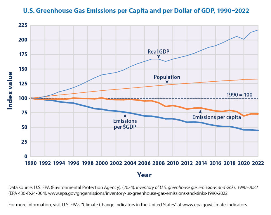
This figure shows trends in greenhouse gas emissions from 1990 to 2022 per capita (heavy orange line), based on the total U.S. population (thin orange line). It also shows trends in emissions per dollar of real GDP (heavy blue line). Real GDP (thin blue line) is the value of all goods and services produced in the country during a given year, adjusted for inflation. All data are indexed to 1990 as the base year, which is assigned a value of 100. For instance, a real GDP value of 217 in the year 2022 would represent a 117 percent increase since 1990.
Let us get to plotting the data.
By the way, we commented out the old URL as new data beame available during the revision.
#url = "https://www.epa.gov/system/files/other-files/2022-07/us-ghg-emissions_fig-3.csv"
url = "https://www.epa.gov/system/files/other-files/2024-06/us-ghg-emissions_fig-3.csv"
df_ghg_percapita = url_data_request(url, 6)

df_ghg_percapita.dtypes
df_ghg_percapita

listcol = df_ghg_percapita.columns.tolist()
listcol.remove('Year')

fig = px.line(df_ghg_percapita, x = 'Year', y = listcol)

fig.update_layout(
    yaxis_title="Index Value (1990=100)",
    title='U.S. Greenhouse Gas Emissions per Capita and per Dollar of GDP, 1990–2021 ', title_x=0.5,
    hovermode="x",
    legend=dict(x=0.2,y=1)
)
fig.update_layout(legend={'title_text':''})
fig.show()
We can plot this data also by making minor modifications to the code that showed earlier. It should be pretty straigh forward by now. We have used a line graph this time (px.line).
From the figure, we can see, as EPA mentions in the key points:
Emissions increased at about the same rate as the population from 1990 to 2007, which caused emissions per capita to remain fairly level (Figure 3). Total emissions and emissions per capita declined from 2007 to 2009, due in part to a drop in U.S. economic production during this time. Emissions decreased again from 2010 to 2012 and continued downward largely due to the growing use of natural gas and renewables to generate electricity in place of more carbon-intensive fuels.
From 1990 to 2022, greenhouse gas emissions per dollar of goods and services produced by the U.S. economy (the gross domestic product or GDP) declined by 55 percent (Figure 3). This change may reflect a combination of increased energy efficiency and structural changes in the economy.